Appendix II – Joint Research Centre (JRC) statistical audit of the 2026 Global Innovation Index

This statistical audit was conducted by Petra Krylova, Jaime Lagüera González, Panagiotis Ravanos, Michaela Saisana, and Oscar Smallenbroek, European Commission, JRC, Ispra, Italy.

Introduction

Robust and reliable monitoring frameworks are essential to better policymaking. As is the case in other socioeconomic fields, understanding and coherently modeling innovation within individual countries, as well as at the global level, is crucial for identifying those emerging trends and best practices that can be used to inform future strategies. Developing and monitoring a framework for innovation presents conceptual and practical challenges such as those related to data quality and choice of methodology. Addressing such challenges is essential for ensuring that policymakers have access to robust and useful information that can be used as input when designing effective innovation policies. This 19^th edition of the Global Innovation Index (GII) 2026 organizes data from 139 economies across 79 indicators into a structured framework of 21 sub-pillars, seven pillars, two sub-indices, and an overall summary index. This appendix delves into the practical challenges of constructing the GII, with the aim of examining the statistical coherence of the conceptual framework and the robustness of the final rankings in relation to the calculations and assumptions from which they are derived.

Statistical coherence should be regarded as a necessary but not sufficient condition for a sound GII, since the correlations underpinning most of the statistical analyses carried out herein need not “necessarily represent the real influence of the individual indicators on the phenomenon being measured” (OECD/EC JRC, 2008OECD/EC JRC (Organisation for Economic Co-operation and Development/European Commission, Joint Research Centre). (2008). Handbook on Constructing Composite Indicators: Methodology and User Guide. Paris: OECD.: 26). Similarly, neither is conceptual clarity alone sufficient, as it does not take into account the measurement quality of the individual indicators, nor how they interact with each other. Therefore, as would be the case for any composite index, developing the GII requires a continuous dialogue between statistical rigor and conceptual understanding, ensuring that empirical data and theory complement each other.

The European Commission’s Competence Centre on Composite Indicators and Scoreboards (CC-COIN) at the Joint Research Centre (JRC) in Ispra, Italy, has been invited to audit the GII for a 16^th consecutive year. As in previous editions, the present JRC-COIN audit focuses on the statistical soundness of the multilevel structure of the index and on the impact of key modeling assumptions on the results, most notably country rankings. ⁽¹⁾The JRC analysis was based on the recommendations of the OECD/EC JRC (2008) Handbook on Constructing Composite Indicators and on more recent research from the JRC. The JRC audits on composite indicators are conducted at the request of the index developers and are available at: https://knowledge4policy.ec.europa.eu/composite-indicators_en and https://composite-indicators.jrc.ec.europa.eu. The independent statistical assessment of the GII provided by the JRC-COIN guarantees the transparency and reliability of the index for both policymakers and other stakeholders alike, thus facilitating more accurate priority setting and policy formulation in the field of innovation.

As in previous GII reports, the JRC-COIN analysis complements the economy rankings of the GII, the Innovation Input Sub-Index and the Innovation Output Sub-Index with confidence intervals, to allow for a better appreciation of the robustness of these rankings in relation to the choice of computation methodology. The JRC-COIN analysis also includes an assessment of the added value of the GII, and it supplements the GII scores with a measure of the “distance to the performance frontier” of innovation using data envelopment analysis.

Source: European Commission, Joint Research Centre, 2026.

Conceptual and statistical coherence within the GII framework

The GII model was assessed by the JRC-COIN in June 2026. Suggestions for fine-tuning certain aspects were communicated to developers during an iterative process with the JRC-COIN aiming to set the foundations for a balanced index. This four-step process is outlined in Box 1.

Step 1: Conceptual consistency

GII 2026 organizes a total of 79 indicators into a hierarchical structure of sub-pillars, pillars, an Input and an Output sub-index, and the final overall index. These were selected as relevant to specific areas of innovation activities based on a literature review, expert opinion, economy coverage and timeliness. To present a fair picture of economies’ differences, indicators were scaled either at source or by the GII team, as appropriate and where needed. For example, Venture capital (VC) received, deal count (indicator 4.2.2) is expressed as number of deals per billion PPP$ GDP, while Researchers (indicator 2.3.1) is expressed as FTE workers per million population. As of 2023 and on the advice of JRC-COIN, the GII developers normalize all 79 indicators to a 0–100 range which facilitates their individual contributions to the overall index score.

The 2026 edition of the GII includes a few changes to the indicators considered.

• The methodology for calculating one indicator (3.3.2 Low-carbon energy use) has changed. In particular, the indicator is now calculated as the share of a country’s total energy supply (expressed in petajoules) that comes from low-carbon intensive sources.

• In sub-pillar 3.2 General infrastructure, a new indicator 3.2.2 Aviation import dwell time has been included. The reason for its inclusion concerns the discontinuation of the World Bank Logistics Performance Index (LPI) in an index format. The new version of the LPI is a dashboard of six indicators based on hard data. Developers selected Aviation import dwell time among those six indicators as most suited. For the current edition of the GII, developers have maintained the Logistics Performance Index as indicator 3.2.3 in the GII framework based on 2024 data (last edition of LPI). This was done to allow for a smooth transition towards full discontinuation of the LPI as a GII component from 2027 onwards. The developers plan to undertake a critical re-assessment of sub-pillar 3.2 in the 2027 edition of the index, with the objective of discontinuing the LPI in its original form.

• Indicator 4.2.5 Joint venture deals (VC investor co-participation per bn PPP$ GDP) has been removed from the 2026 framework. This indicator was highly correlated with indicator 4.2.4 VC investors. Developers selected the latter as more relevant to avoid the potential double counting of information in the overall index resulting from highly correlated components.

• Finally, in sub-pillar 5.3 Knowledge absorption, indicator 5.3.5. Green-field R&D & high-tech FDI has been introduced to the framework. The reason is conceptual: developers opted for reinforming the measurement of FDI by also looking at the announced investments in specific R&D and high-tech projects.

The above changes highlight the developers’ commitment to rigorously monitoring, evaluating, and refining the theoretical framework and the data sources underpinning the index, both from a conceptual and statistical point of view. This continuous improvement process ensures that the index delivers a reliable, accurate and timely assessment of innovation performance that provides policymakers with reliable insights to drive evidence-based decision-making.

Step 2: Data checks

The data used for each economy were those most recently released within the period 2016 to 2026. Also, more than 95 percent of the available data refers to 2022 or a later year. With regards to the inclusion of countries in the GII, the 2026 edition follows the criteria adopted in 2016, ⁽³⁾These criteria were adopted following a JRC-COIN recommendation based on previous GII audits. according to which economies are only included if (i) data availability is at least 66 percent within each of the two sub-indices (i.e., 36 out of 54 variables within the Input Sub-Index and 17 out of the 25 variables in the Output Sub-Index) and (ii) at least two of the three sub-pillars in each pillar can be computed. These criteria aim to ensure that economy scores for the GII and for the two Input and Output Sub-Indices are not overly sensitive to missing values (as was the case for the Output Sub-Index scores of several economies in previous editions). In the current edition of the Index, three additional countries fulfill these criteria compared to the previous iteration (Bhutan, Democratic Republic of Congo, and Chad) and are thus added to the GII 2026, while three other countries failed to fulfill the criteria and were excluded from this year’s iteration (Congo, Guinea, Seychelles). Thus, the number of economies is the same as in the previous version of the index (139).

In practice, data availability for all economies included in the GII 2026 is quite satisfactory: at least 80 percent of data is available for 77 percent of the economies covered (equivalent to 107 economies out of 139), while 84 percent of the considered indicators are available for at least 75 percent of the 139 economies covered. This highlights the significant efforts conducted by the GII in promoting continuous data monitoring and collection in the realm of innovation-related variables. There are only two indicators for which the share of missing data is relatively high: indicator 4.1.3 Loans from microfinance institutions and indicator 7.2.3 Entertainment and media market, for which data are available for 47 percent and 46 percent of the 139 countries respectively. JRC-COIN would like to suggest that developers keep these two indicators under closer scrutiny for the next iterations of the GII and investigate the potential of increasing their data availability.

Data quality checks by the JRC-COIN team also consider the properties of data distributions, and the skewness and kurtosis, which flag indicators with reduced ability to differentiate between countries. In 2011, a joint decision by the GII team and the JRC-COIN determined that values would be treated if an indicator had absolute skewness greater than 2.0 and kurtosis greater than 3.5. ⁽⁴⁾Groeneveld and Meeden (1984)Groeneveld, R.A. and G. Meeden (1984). Measuring skewness and kurtosis. The Statistician, 33(4), 391–399. set the criteria for absolute skewness above 1 and for kurtosis above 3.5. The skewness criterion was relaxed in the GII case after ad hoc tests were conducted in the GII 2008–GII 2018 series range. In 2017, having analyzed data in the GIIs compiled between 2011 and 2017, less stringent criteria were adopted. An indicator was only treated if the absolute skewness was greater than 2.25 and kurtosis greater than 3.5. Such indicators were treated either by winsorization or by natural logarithm (in cases of more than five outliers; see Appendix I). In 2018, exceptional behavior by foreign direct investment (FDI) net outflows (indicator 6.3.4 at the time) was observed (Annex 3, JRC Audit, GII 2018) and, from 2018 onward, it was recommended that the GII rule for the treatment of outliers be amended as follows:

• for indicators with absolute skewness greater than 2.25 and kurtosis greater than 3.5, apply either winsorization or the natural logarithm (in cases of more than five outliers);

• for indicators with absolute skewness less than 2.25 and kurtosis greater than 10.0, produce scatterplots to identify potentially problematic values that need to be considered as outliers and treated accordingly.

For a total of 32 indicators, one up to five values were winsorized, while for an additional nine indicators (2.3.3 Global corporate R&D investors, 4.2.3 Late-stage VC deal count, 4.3.3 Domestic market scale, 5.2.5 Patent families, 6.1.1 Patents by origin, 6.3.1 Intellectual property receipts, 7.1.4 Industrial designs by origin, 7.2.4 Creative goods exports, and 7.3.3 Mobile app creation) the natural logarithm was applied. For two of these five indicators (4.2.3 Late-stage VC deal count and 5.2.5 Patent families) the values of skewness and kurtosis did not abide by the set thresholds after applying the natural logarithm transformation.

Compared to the previous edition of the GII in 2025, there were two less indicators that needed a natural logarithm treatment (nine versus 11 last year). The JRC guidelines for data treatment are governed by the principle of least intervention. Therefore, winsorization is preferred as a first treatment followed by natural logarithm transformation. To reduce the indicators treated by the natural logarithm, the JRC would like to suggest increasing the number of maximum winsorized data points for the GII indicators by two from five to seven. This corresponds to the upper 5 percent (7/139) of the distribution with 139 countries, that is to say, values are trimmed up to the 95 percent percentile (if needed). Tests conducted by the JRC indicate that increasing the number of winsorized points would eliminate the need to apply the natural logarithm to six of the nine indicators. For the remaining three indicators (2.3.3 Global corporate R&D investors, 6.1.1 Patents by origin, and 6.3.1 Intellectual property receipts) the logarithmic transformation is already sufficient to bring skewness and kurtosis values within the recommended thresholds.

Step 3: Statistical coherence

Weights as scaling coefficients

The JRC-COIN and the GII team jointly decided in 2012 that weights of 0.5 or 1.0 were to be used as scaling coefficients and not importance coefficients, with the aim of arriving at sub-pillar and pillar scores that were balanced in their underlying components (i.e., that indicators and sub-pillars can explain a similar amount of variance in their respective sub-pillars/pillars). ⁽⁵⁾In this context, a weight of 0.5 does not mean that the corresponding indicators are multiplied by a weight of 0.5 per se, but that an indicator receives half (0.5 or 50 percent) of the maximum weight allocated within its aggregation level. The “nominal’ weight is then obtained by dividing the scaling coefficients by their sum. So, in a hypothetical pillar with three indicators, two of which get a scaling coefficient of 1.0 and the third gets a coefficient of 0.5, the third indicator’s nominal weight (0.2 = 0.5/(0.5 +1+1)) is half of the nominal weight of the other two indicators 0.4 = 1.0/(0.5 +1+1)). In weighted arithmetic averages, the ratio of two nominal weights gives the rate of substitutability between two indicators (see, e.g., Becker et al. (2017)Becker, W., M. Saisana, P. Paruolo and I. Vandecasteele (2017). Weights and importance in composite indicators: Closing the gap. Ecological Indicators, 80, 12–22. and Paruolo et al. (2013)Paruolo, P., M. Saisana and A. Saltelli (2013). Ratings and rankings: Voodoo or science? Journal of the Royal Statistical Society, A 176(3), 609–634.), and hence can be used to reveal the relative importance of individual indicators. This importance can then be compared with ex-post measures of a variable’s importance, such as the non-linear Pearson correlation ratio.

Three additional indicators are slightly unbalanced and fall just below the inclusion threshold. Specifically, SP1.1 and SP1.2 are highly correlated with P1, with correlation coefficients just below the 0.95 cutoff, while the correlation of SP1.3 with P1 is below 0.80. Based on the current contribution of these sub-pillars to the pillar, the developers may also consider applying a scaling coefficient of 0.5 to improve balance across the sub-pillars, which would result in a correlation around 0.80 between all sub-pillars and pillars.

As a result of this analysis, two indicators (1.2.1 Regulatory quality, 1.2.2 Rule of law) and two sub-pillars (7.2 Creative goods and services and 7.3 Online creativity) are given a weight of 0.5.

Despite this weighting adjustment, three indicators (3.2.4 Gross capital formation, 5.3.4 FDI net inflows and 6.2.1 Labor productivity growth) were found to be non-influential in this year’s GII framework, meaning that they could not explain at least 9 percent of economies’ overall variation in the respective sub-pillar scores (see Appendix II Table 1).

These three indicators also remain statistically non-influential at both the sub-index and the index level, while there are five additional indicators (2.1.1 Expenditure on education, 2.2.2 Graduates in science and engineering, 3.3.2 Low-carbon energy use, 4.1.3 Loans from microfinance institutions, 7.2.2 National feature films) which are not sufficiently correlated with the (Input or Output) Sub-Index level as well as the GII itself. This means that, at least for 3.2.4 Gross capital formation, 5.3.4 FDI net inflows and 6.2.1 Labor productivity growth, there is evidence of a weak relationship between a country’s GII index scores and its Gross capital formation, FDI net inflows or Labor productivity growth.

As previously noted, a weak statistical relationship does not imply that an indicator is conceptually unsuitable. Rather, it reflects the amount of information (or variability) that the indicator contributes to the overall index. This is given by the squared Pearson correlation coefficients in Appendix II Table 1. Specifically, the weak correlation between the Gross capital formation, FDI net inflows, and Labor productivity indicators and the GII indicates only a limited relationship, without suggesting any causality or its absence. The JRC-COIN encourages the developers to carefully monitor the statistical fit of these indicators in future editions of the index and to thoughtfully assess their impact on economies most affected by their inclusion in the framework.

The indicator 5.1.3 Youth demographic dividend warrants special attention. The indicator’s statistical fit with the remaining GII variables is rather peculiar: it shows a statistically significant negative correlation (< –0.4) with all other indicators within the sub-pillar 5.1 Knowledge workers, as well as with the GII index, with which it has a negative correlation coefficient of –0.76. Similarly, weak correlations are observed with many other indicators across the GII framework – 64 out of 77 indicators show a negative correlation below –0.3 with this indicator.

As JRC-COIN has noted previously (Laguera-Gonzalez et al., 2025Lagüera González, J., Ravanos, P., Saisana, M., Smallenbroek, O., Guidi, A., and Borrega A.C. (2025). Appendix II-Joint Research Centre (JRC) Statistical audit of the 2025 Global Innovation Index. In: World Intellectual Property Organization (WIPO). Global Innovation Index 2025: Innovation at a Crossroads, 2025, pp. 245-266. Geneva: WIPO. https://doi.org/10.34667/tind.58864), this indicator has a pronounced regional impact, as it tends to favor African countries by effectively providing a “bonus” that reflects their unique demographic advantage. The youthful populations in many African economies position them with significant potential for innovation and economic growth in the years ahead, driven by their expanding youth population that could transform into valuable human capital. This regional dimension highlights the indicator’s role in capturing forward-looking potential innovation capacity that may not be fully reflected by other measures in the index. While the JRC-COIN acknowledges the conceptual reasoning for including this indicator and its future-oriented nature, it comments the following on its statistical fit within the GII framework: the strong negative correlations observed can reduce the framework’s ability to effectively differentiate and rank countries and increase sensitivity to weighting choices. Therefore, the JRC-COIN echoes its suggestion in the previous Audit (Laguera-Gonzalez et al., 2025Lagüera González, J., Ravanos, P., Saisana, M., Smallenbroek, O., Guidi, A., and Borrega A.C. (2025). Appendix II-Joint Research Centre (JRC) Statistical audit of the 2025 Global Innovation Index. In: World Intellectual Property Organization (WIPO). Global Innovation Index 2025: Innovation at a Crossroads, 2025, pp. 245-266. Geneva: WIPO. https://doi.org/10.34667/tind.58864) and encourages the developers to further delve into the insights provided by the Youth demographic dividend indicator in the GII framework and to carefully consider retaining the indicator as a critical but contextual component in future index editions – particularly for its value in highlighting the innovation potential of regions with youthful demographic profiles, such as Africa.

The remaining 70 indicators out of the 79 in total were found to be sufficiently influential – in the statistical sense – in the GII framework.

Principal component analysis and reliability item analysis

Principal component analysis (PCA) was used to assess the extent to which the conceptual framework is confirmed by statistical approaches. PCA results confirm the presence of a single latent dimension in each of the seven pillars (one component with an eigenvalue greater than 1.0) that captures between approximately 68 percent (pillar 3: Infrastructure) and up to 80 percent (pillar 1: Institutions) of the total variance in the three underlying sub-pillars. Furthermore, results confirm the expectation that in the vast majority of cases, the sub-pillars are more closely correlated with their own pillar than with any other pillar and that nearly all correlation coefficients are greater than 0.70 (with the exception of 3.3 Ecological sustainability 0.69), suggesting that each sub-pillar’s variation can explain at least 50 percent of the variation in its parent pillar (Appendix II Table 2).

The five input pillars share a single statistical dimension that summarizes 81 percent of the total variance, and the five loadings (correlation coefficients) of these pillars are very similar to each other. This similarity suggests that the five pillars make a roughly equal contribution to the variation of the Innovation Input Sub-Index scores, as envisaged by the development team. Consequently, the reliability of the Input Sub-Index, measured by Cronbach’s alpha value, is very high at 0.93 – well above the 0.70 threshold for a reliable aggregate (Nunally, 1978Nunally, J. (1978). Psychometric Theory. New York: McGraw-Hill.).

The two output pillars – Knowledge and technology outputs and Creative outputs – are strongly correlated with each other (0.88); they are also both strongly correlated with the Innovation Output Sub-Index (0.96 and 0.97, respectively). As expected, the reliability of the Output Sub-Index, measured by Cronbach’s alpha value, is also very high (0.93).

Finally, the two sub-indices are equally important in the overall GII. The GII is built as a simple arithmetic average of the Input Sub-Index and the Output Sub-Index. In fact, the Pearson correlation coefficients of the two sub-indices with the GII (around 0.97 in both cases), and the correlation between themselves (0.90), suggests that they are effectively placed on an equal footing.

Added value of the GII

The strong statistical association between the components of a composite index could also signal potential redundancy (or double counting) of information within the composite index. For the case of the GII, the Input and Output Sub-Indices correlate strongly with each other and with the overall GII, while the pillars in the Input and the Output Sub-Indices have a very high statistical reliability. However, analysis conducted by the JRC-COIN on country rankings based on these aggregates confirms that this high statistical reliability does not result in redundancy of information. A country’s GII ranking differs from that in any of its seven pillars by 10 positions or more for at least 45 percent (up to 72 percent) of the 139 economies included in the GII 2026 (Appendix II Table 3). Similarly, the average change in country ranks (Saisana et al., 2005) between any pillar and the GII is at least 10.5 rank positions (Creative outputs) and up to 21 rank positions (Institutions). This serves as a demonstration of the added value of the GII ranking, which helps to highlight other aspects of innovation within individual countries that are not immediately apparent from analysis of the seven pillars individually. It also highlights the usefulness of taking due account of the information contained in each of the GII pillars, sub-pillars and indicators individually. By doing so, economy-specific strengths and bottlenecks in innovation inputs, framework conditions, and outputs can be identified and serve as a basis for evidence-based policymaking.

Step 4: Qualitative Review

Lastly, JRC-COIN evaluated the GII results – in particular, the overall economy classifications and relative performances in terms of the Innovation Input or Output Sub-Indices – with the aim to verify that the overall results are robust with respect to the modeling assumptions made during the development of the GII.

The impact of modeling assumptions on the GII results

Any composite index, the GII included, is the result of methodological choices made along the way during its development. In many cases, such choices have a clear rationale, but there is always some equally plausible alternative that could be also chosen. The existence of such alternatives creates an inherent uncertainty in composite index scores and rankings, as these are likely to differ each time a different methodological choice is made. A powerful characteristic of a composite index is that the information it conveys (notably, country rankings) is robust to these alternative methodological choices. Robustness verifies its reliability as a monitoring framework of the underlying phenomenon that is being measured. Overall, the results in this section verify the robustness of the GII with respect to modeling assumptions and its reliability as a monitoring framework for innovation performance at the global level. Notwithstanding these positive results, the structure of the GII model is, and must remain, open to future improvements which may be needed as better data, more comprehensive surveys and assessments, and new, relevant research studies become available.

An important part of the GII statistical audit is to check the potential effect of varying methodological choices made while developing the GII within plausible ranges.

Modeling assumptions with a direct impact on GII scores and rankings relate to:

• the underlying structure selected for the index based on pillars;

• the choice of individual variables to be used as indicators;

• decisions regarding whether (and how) to impute missing data;

• decisions regarding whether (and how) to treat outliers;

• the selection of the normalization formula to be used;

• the choice of aggregation weights for indicators and their aggregates; and

• the aggregation rule to be used at each different level of the index structure.

The rationale for the choices made by the GII developers regarding each of these issues is well-grounded: for instance, expert opinion coupled with statistical analysis informs the selection of the individual indicators; common practice and easier interpretation suggest the use of a minimum–maximum normalization approach in the [0–100] range; statistical analysis guides the treatment of outliers; while simplicity and parsimony criteria advocate for the developers’ choice for not imputing missing data. The uncertainty that naturally stems from the above-mentioned modeling choices is accounted for in the robustness assessment carried out by the JRC-COIN. In particular, the methodology applied allows for the joint and simultaneous analysis of the impact made by such choices on the aggregate scores. The analysis carried out by JRC-COIN supplements the GII 2026 individual economy rankings with confidence intervals, to better appreciate the robustness of these rankings in relation to the modeling choices.

As suggested by the relevant literature on composite indicators (Saisana et al., 2005Saisana, M., A. Saltelli and S. Tarantola (2005). Uncertainty and sensitivity analysis techniques as tools for the analysis and validation of composite indicators. Journal of the Royal Statistical Society, A 168(2), 307–323.; Saisana et al., 2011Saisana, M., B. D’Hombres and A. Saltelli (2011). Rickety numbers: Volatility of university rankings and policy implications. Research Policy, 40(1), 165–177.; Vertesy, 2016Vertesy, D. (2016). A Critical Assessment of Quality and Validity of Composite Indicators of Innovation. Paper presented at the OECD Blue Sky III Forum on Science and Innovation Indicators. Ghent, 19–21 September 2016.; Vertesy and Deiss, 2016Vertesy, D. and R. Deiss (2016). The Innovation Output Indicator 2016: Methodology Update, EUR 27880. Luxembourg: European Commission, Joint Research Centre.; Montalto et al., 2019Montalto, V., C.J. Tacao Moura, S. Langedijk and M. Saisana (2019). Culture counts: An empirical approach to measure the cultural and creative vitality of European cities. Cities, 89, 167–185.) the robustness assessment is based on Monte Carlo simulation and multi-modeling approaches, applied to data that are assumed to be “error-free” where potential outliers, errors and typos have already been corrected at a preliminary stage. In particular, the three key modeling issues considered in the assessment of the GII were the treatment of missing data, the aggregation formula and weights applied to the pillar level.

The Monte Carlo simulation comprised 5,000 runs of different sets of weights for the seven GII pillars. Weights were assigned to the pillars based on random perturbations centered on the reference values. The ranges of simulated weights were defined by considering both the need for a wide enough interval to allow for meaningful robustness checks and the need to respect the underlying principle of the GII that the Input and the Output Sub-Indices should be placed on an equal footing. As a result of these considerations, the limit values of uncertainty for the five input pillars are between 10 and 30 percent, whereas the limit values for the two output pillars are between 40 and 60 percent (Appendix II Table 4).

For transparency and replicability purposes, the GII team has always opted not to estimate missing data. In cases where missing data exists, the score of the aggregate containing the missing value is based on the other elements of the aggregate for which values are observed. This “no imputation” choice is common in other composite indicators and is usually selected to improve transparency and avoid any methodological black box in the imputation of data. Technically, this constitutes a form of “shadow” imputation (for example, in an arithmetic average it is equivalent to replacing the missing value with the arithmetic average of the elements for which values are observed). Hence, the available data (indicators) in the incomplete pillar may dominate it, sometimes biasing the ranks up or down. To test the impact of not imputing missing values, the JRC-COIN estimated missing data using two different data imputation approaches: (a) the expectation–maximization (EM) algorithm and (b) the k-nearest neighbor (k-NN) approach (using the 10 nearest neighbors). Both were applied within each GII pillar and then compared to the no-imputation approach (see Appendix II Table 6). ⁽⁶⁾The expectation–maximization (EM) algorithm (; ) is an iterative procedure that finds the maximum likelihood estimates of the parameter vector by repeating two steps: (a) The expectation step (E-step): given a set of parameter estimates, such as a mean vector and covariance matrix for a multivariate normal distribution, the E-step calculates the conditional expectation of the complete-data log likelihood, given the observed data and the parameter estimates. (b) The maximization step (M-step): given a complete-data log likelihood, the M-step finds the parameter estimates to maximize the complete-data log likelihood from the E-step. The two steps are iterated until the iterations converge. The k-nearest neighbor approach replaces a missing value for a country A with the average of the values observed for the same indicator in k (which in this case is equal to five) other sample countries which are identified as country A’s “nearest neighbors,” in the sense that their performance in the other indicators is similar to that of country A. This involves two steps: (a) estimating measure of distance between country A and all other sample countries (e.g., the Euclidean distance) based on the indicators for which country A has observed data and selecting the k countries with the smaller distance to country A, and (b) obtaining the average of the indicator values for the selected countries and using it to fill the missing value for country A.

With regards to the aggregation formula, decision theory practitioners challenge the use of simple arithmetic averages because of their fully compensatory nature, where a country’s high comparative advantage on a few indicators can compensate for its comparative disadvantage on many other indicators (Munda, 2008Munda, G. (2008). Social Multi-Criteria Evaluation for a Sustainable Economy. Berlin and Heidelberg: Springer-Verlag.). To assess the impact of this modeling choice, the JRC-COIN explored various scenarios of the weighted generalized mean ⁽⁷⁾The various scenarios for the generalized mean involve using different exponent values: 0, 0.25, 0.75, and 0.5, allowing for various levels of compensability. In the geometric average (exponent value = 0), pillars are multiplied as opposed to summed in the arithmetic average. Pillar weights appear as exponents in the multiplication. All pillar scores were greater than zero, hence there was no reason to rescale them to avoid zero values that would have led to zero geometric averages. as an alternative to the arithmetic average. These scenarios allow less compensability, ⁽⁸⁾To elaborate more on the limited compensability under different p values, assume two components A and B being aggregated into a composite index with equal weights, where A = 0.5 × B. If p = 1 (arithmetic mean), a decline in A (the component in which performance is worse and in fact half that of B) of 1 unit will cause the same decline in the composite index as a decline in B (the component in which performance is two times larger) by 1 unit (perfect compensability). This is because the relative impact of an increase in A compared to B is equal to (A/B)^a-1. If p = 0.75, 0.5, or 0.25, the decline in A will cause a decline in the composite index which will be about 1.18, 1.41, and 1.68 times larger, respectively, compared to a decline in B by the same amount, while when p → 0 (geometric mean) the decline in A will cause a decline in the composite index which will be 2 times larger compared to a decline in B by the same amount (see the discussion on the properties of the generalized mean in UNDP, 1997UNDP (United Nations Development Programme) (1997). Human Development Report 1997. New York: Oxford University Press.). rewarding economies with balanced profiles and encouraging them to improve in the GII pillars in which they perform poorly, rather than just excelling in any GII pillar.

Fifteen models were tested based on the combination of no imputation versus EM or k-NN imputation and arithmetic versus generalized average, with the geometric average being the variation of the generalized average that allows the least compensability among those tested. A random combination of these choices plus a random set of perturbed weights were used in a total of 5,000 simulations for the GII and each of the two sub-indices (see Appendix II Table 4 for a summary of the uncertainties considered).

Uncertainty analysis results

The main results of the robustness analysis are shown in Appendix II Figure 1, with median ranks and 90 percent confidence intervals computed across the 5,000 Monte Carlo simulations for the GII and the two sub-indices. Economies are in ascending order (best to worst performing) according to their reference rank (solid straight line), with the dot representing the median rank over the simulations.

Appendix II Figure 1 Robustness analysis of the GII, Input and Output Sub-Indices

As is evident, all published GII 2026 ranks lie within the simulated 90 percent confidence intervals. Furthermore, for most economies these intervals are sufficiently narrow to allow meaningful inferences to be drawn with regard to each economy’s relative standing in terms of innovation performance: the width of the 90 percent GII rank confidence interval is less than 10 positions in rank for 86 of the 139 economies considered in the GII (62 percent), while this holds for 103 of the 139 economies in the case of the Input Sub-Index and for 110 in the case of the Output Sub-Index. This suggests a significant robustness of the GII and its sub-indices to effectively discriminate between the economies ranked even if various methodological choices change. However, it is also true that a small group of economies experience significant changes in rank with variations in weights and aggregation formula and when imputing missing data. Two economies – Brunei Darussalam and Madagascar – have 90 percent confidence interval widths of more than 20 positions (27 and 42 positions, respectively). Consequently, their rankings (98th and 113th) in the GII classification should be interpreted cautiously and not taken at face value. However, this is a remarkable improvement compared to GII versions up to 2016, when more than 40 economies had confidence interval widths of more than 20 positions. The improvement in confidence intervals in the GII 2026 ranking is the direct result of the decision to adopt a more stringent criterion for an economy’s inclusion since 2016, which now requires at least 66 percent data availability within each of the two sub-indices. There is also an improvement compared to the previous version of the GII in 2025, in which seven economies realized confidence intervals larger than 20 positions.

Similarly, some caution is also warranted with regards to the ranking of three economies (Belarus, Bhutan and Paraguay) for the Input Sub-Index, for which the 90 percent confidence interval has a width of more than 20 positions (22, 29 and 24, respectively). In the Output Sub-Index, this occurs for four economies – Bhutan, Ghana, Lebanon and Madagascar – for which the 90 percent confidence interval widths are up to 29 positions. The higher data availability in the Output Sub-Index in the latest GII editions has contributed to reducing the number of countries with very wide intervals compared to previous editions (e.g., the GII 2019 edition in which there were 13 countries with confidence intervals wider than 20 positions).

Although the rankings for a few economies in the GII or in the two sub-indices appear to be sensitive to methodological choices, the published rankings for the vast majority of the 139 countries included in the 2026 GII and its two sub-indices can be considered as representative of the plurality of scenarios simulated in this audit. Taking the median simulated rank from the Monte Carlo uncertainty analysis as the benchmark for an economy’s expected rank in the realm of the GII’s unavoidable methodological uncertainties, 69 percent of the economies are found to shift fewer than three positions with respect to the published rank in the GII; the percentage for the Input and the Output Sub-Indices is similarly large (at 59 and 68 percent, respectively).

To offer full transparency and complete information, Appendix II Table 5 reports the GII 2026 Index and Input and Output Sub-Indices’ economy ranks together with the simulated 90 percent confidence intervals to allow a better appreciation of the robustness of the results to the choice of weights, aggregation formula and the impact of estimating missing data (where applicable).

Sensitivity analysis results

Complementary to the uncertainty analysis, sensitivity analysis has been used to identify which of the modeling assumptions have the greatest impact on certain country rankings. Appendix II Table 6 summarizes the impact of one-off changes in the imputation method (no imputation versus EM or k-NN imputation) and/or the aggregation formula (arithmetic versus generalized aggregation), keeping the aggregation weights fixed at their reference values (as in the nominal GII). As with the results of previous audits, neither the GII nor the Input or Output Sub-Indices are found to be heavily influenced by the imputation of missing data, or by the aggregation formula. Regarding the GII index, there is only one economy (Brunei Darussalam) for which rank deteriorates by more than 20 positions when generalized aggregation is used instead of arithmetic aggregation. On the other hand, Bhutan’s Input Sub-Index rank deteriorates by more than 20 positions when a combination of a different aggregation and imputation method is used (generalized aggregation and k-NN). The choice of the imputation method appears to also be crucial for the ranking of three other countries in the case of the Output Sub-Index, namely Ghana, Nicaragua and Zimbabwe. For these countries, missing data account for 16, 32, and 4 percent of the Output Sub-Index indicators. ⁽⁹⁾Zimbabwe is missing data for indicator 7.2.3 only. However, the normalized values of the remaining three indicators within sub-pillar 7.2 are very low (less than 3 with 100 being the best performance) and hence their average – which is implicitly assigned to indicator 7.2.3 in the nominal GII – is similarly low. The alternative imputation methods are based also on the data of similar countries to impute indicator 7.2.3, potentially resulting in much larger values than the average.

Overall, the analysis carried out by JRC-COIN verifies that the rankings of the 2026 GII are reliable and, for the vast majority of the considered economies, the simulated 90 percent confidence intervals are narrow enough to allow meaningful inferences to be drawn for their relative performance. There are a few economies that appear to be sensitive to the way missing values are treated, most of which have a rather large share of missing data. It is however suggested that the readers of the GII 2026 report consider an economy’s ranking in the GII 2026 and in the Input and Output Sub-Indices not only at face value, but also within the 90 percent confidence intervals, to better appreciate the degree to which an economy’s rank depends on modeling choices.

Best-practice frontier in the GII by data envelopment analysis

Can we benchmark economies’ multidimensional innovation performance without applying a fixed and uniform set of weights that might be unfair to a particular economy?

Indicator developers often face this question, particularly when stakeholders feel that the selection of aggregation weights might not reflect their current trajectory and future aspirations. Indeed, innovation policies at the national level must strike a balance between global trends that need to be followed (such as lately the adoption of AI) and each country’s unique context (e.g., development stage), future strategies (e.g., how they inspire to adopt AI), and challenges that lie ahead. Evaluating multidimensional innovation performance by applying a common set of weights to all economies could hinder the acceptance of an innovation index, as the chosen weighting scheme might be perceived as unfair to specific economies since it does not reflect their national priorities or the distinct challenges they encounter compared to other economies. Scholars have indicated that composite indices could use country-specific weights to reflect such country specificities (see, e.g., Srinivasan’s (1994)Srinivasan, T.N. (1994). Human development: A new paradigm or reinvention of the wheel? American Economic Review, 84, 238–243. note on the Human Development Index). A notable advantage of data envelopment analysis (DEA), as applied in real world decision-making contexts, is exactly this feature. It endogenously determines a set of aggregation weights that optimize each economy’s overall composite score, given a set of other observations (economies). In the absence of a global consensus or strategy on innovation activity priorities, and with numerous national innovation strategies influenced by diverse country-specific factors, this approach presents a reasonable alternative to using uniform weights across economies.

In this section we relax the assumption of fixed pillar weights common to all economies by allowing economy-specific weights that maximize an economy’s global innovation score to be determined endogenously by means of the Benefit-of-the-Doubt (BoD) model, a tailored DEA model that is suitable for the case of composite indicators construction. The original question posed by the DEA literature was how to measure each unit’s relative efficiency in production compared to a sample of peers, given observations on input and output quantities and, often, no reliable information on prices (Charnes and Cooper, 1985Charnes, A. and W.W. Cooper (1985). Preface to topics in data envelopment analysis. Annals of Operations Research, 2, 59–94.). A notable difference between the original DEA approach and the one of the BoD model that is used here is that no differentiation between inputs and outputs is made but instead only outputs (indicators) are considered (Cherchye et al., 2008Cherchye, L., W. Moesen, N. Rogge, T. Van Puyenbroeck, M. Saisana, M. et al. (2008). Creating composite indicators with DEA and robustness analysis: The case of the Technology Achievement Index. Journal of Operational Research Society, 59(2), 239–251.). Thus, along the lines of Cook et al., (2014)Cook, W.D., K. Tone and J. Zhu (2014). Data envelopment analysis: Prior to choosing a model. Omega, 44, 1–4. the BoD model evaluates countries with respect to a best-practice frontier formed by the countries with the relatively best achievements in the considered pillars, rather than an efficiency frontier formed by the countries that transform inputs to outputs in the most efficient way. One can view this as a special kind of "production" process where each economy employs an apparatus of socioeconomic norms, rules and strategies to steer its innovation performance to the maximum possible (Lovell et al., 1995Lovell, C.A.K., J.T. Pastor and J.A. Turner (1995). Measuring macroeconomic performance in the OECD: A comparison of European and non-European countries. European Journal of Operational Research, 87(3), 507–518.).

To estimate DEA-BoD-based distance to the best-practice frontier scores, we consider the m = 7 pillars in the GII 2026 for n = 139 economies, with y_ij the value of pillar j in economy i. The objective is to combine the pillar scores per economy into a single number, calculated as the weighted average of the m pillars, where w_j represents the weight of the j-th pillar. In the absence of reliable information about the true weights, the weights that maximize the DEA-BoD-based scores are endogenously determined. This gives the following linear programming problem for each economy i:

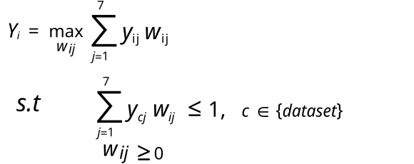
where, j = 1,…, 7, i = 1,…, 139 (non-negativity constraint). In this linear programming problem, the weights are non-negative and an economy’s score is between 0 (worst) and 1 (best). The programming problem used to calculate the DEA-BoD scores in this audit included also the restrictions: 0.2 ≥ (w_ij*y_ij)/Σ(w_ij*y_ij) ≥ 0.05, j = 1,…, 7 (contribution restrictions).

In theory, each economy is free to decide on the relative weight of each innovation pillar, such as to achieve the best possible score, allowing for a better reflection of its unique innovation strategy. In practice, the DEA-BoD method assigns a higher (lower) weight to those pillars in which an economy is relatively strong (weak). Reasonable constraints are applied to the weights to preclude the possibility of an economy achieving a perfect score by assigning a zero weight to weak pillars: for each economy, no pillar can contribute less than 5 percent or more than 20 percent to an economy’s total score. This is imposed by including the restrictions: 0.2 ≥ (w_ij*y_ij)/Σ(w_ij*y_ij) ≥ 0.05, j = 1,…, 7 (contribution restrictions) to the above linear program. The DEA-BoD score is then calculated as a weighted average of the seven innovation pillar scores, using the economy-specific weights determined by the DEA-BoD method. This score is compared to the best performance among all other economies using the same weights. The DEA-BoD score can be interpreted as a measure of the “distance to the best-practice frontier.”

Appendix II Table 7 presents pie shares, DEA-BoD scores and rankings for the top 25 economies in the GII 2026 alongside their respective GII 2026 rankings. All pie shares are in accordance with the starting point of granting leeway to each economy when assigning shares, while not violating the (relative) upper and lower bounds. Switzerland is the only economy to obtain a perfect DEA-BoD score of 1.00 after the weight restrictions are included – indicating that it defines the best-practice frontier (in past GII versions, other economies were identified as best-practice as well). Sweden (0.99), Singapore (0.98), the United States (0.97), the Republic of Korea (0.96) and Finland (0.94) follow in terms of relative performance. The scores of these countries indicate that they are very close to the best-practice frontier: a proportional improvement of their pillar scores by 1 percent (1/0.99 = 1.01) to 6 percent (1/0.94 = 1.06) would make them frontier economies as well.

The seven pillars contribute differently to the performance scores of the top 25 economies, mirroring the varied priorities in their national innovation strategies. These differences also highlight each economy’s strengths in specific GII pillars compared to others, revealing their comparative advantages. For instance, France and Canada obtain the same performance score (0.85) but France relies less on Institutions and more on Creative outputs to do so. In a similar fashion, the United States and the Republic of Korea receive roughly the same score (0.97 and 0.96, respectively), but their pillars contribute differently to it: both countries allocate 20 percent – the maximum possible – of their score to Human capital and research and Business sophistication, in which both are very well-performing. However, the United States allocates another 20 percent on the Market sophistication and Knowledge and technology outputs pillar, while the Republic of Korea allocates more weight on the Infrastructure and Creative outputs pillars. Appendix II Figure 2 shows how close the DEA-BoD scores and the GII 2026 scores are for all the 139 economies (Pearson correlation of 0.994). ⁽¹⁰⁾This closeness between the DEA-BoD and the GII scores is, to some extent, a result of the contribution restrictions introduced into the DEA-BoD model. These restrictions are necessary to avoid countries putting zero weights to certain pillars and to allow for a reasonable leeway for countries to perturb weights around the nominal GII weights. For one country – the Bolivarian Republic of Venezuela – the DEA-BoD score is lower than the (rescaled) GII score because the restrictions appended in the DEA-BoD model to restrict the contribution of each of the seven pillars to no less than 5 percent and no more than 20 percent result in the country selecting a set of aggregation weights that is less favorable compared to the nominal GII weights. This is mostly due to the Institutions and Human capital and research pillars, which make up 1.5 percent and 29.3 percent, respectively, of the country’s nominal GII, while in the BoD recalculation their share is respectively 5 percent and 20 percent due to the upper and lower bound restrictions.

Conclusion

The JRC-COIN analysis confirms that the multilevel structure of the GII 2026, encompassing 79 indicators, 21 sub-pillars, seven pillars and two sub-indices, is statistically robust and well-balanced. Each sub-pillar contributes similarly to the variation within its respective pillar, ensuring a framework where conceptual coherence goes hand-in-hand with statistical coherence. The continuous refinements of the conceptual framework by the development team strengthen the GII’s statistical integrity, with most indicators effectively distinguishing between economies’ performances at the sub-pillar level or lower.

The decision not to impute missing values, which is common in comparable contexts and justified on the grounds of transparency and replicability, can at times have an undesirable impact on some economies’ scores, with the additional negative side-effect that it might encourage economies not to report low data values. The GII team’s adoption, in 2016, of a more stringent data coverage threshold (at least 66 percent data availability for each of the input- and output-related indicators) has notably improved confidence in the economy ranking for the GII and the two sub-indices. The results of the analysis carried out by JRC-COIN suggest that the developer’s decision not to impute missing values has a notable impact on the rankings of only a very small set of countries and only in the case of the Input or the Output Sub-Indices. Notably, only five countries exhibit a change in their rank of more than 20 positions when alternative imputation and aggregation methods are applied to the GII 2026.

Additionally, the GII team’s decision, in 2012, to use weights as scaling coefficients during index development constitutes a significant departure from the traditional, yet erroneous, vision of weights as a reflection of indicators’ importance in a weighted average. It is hoped that such an approach will be adopted by other developers of composite indicators to avoid situations where bias sneaks in when least expected.

The correlation structure of the GII framework is statistically sound. In fact, most indicators (70 out of the 79) are found to be sufficiently influential – in a statistical sense – in the GII framework. This result shows the efforts made by the GII team over the past two decades to prepare and continuously update the monitoring framework that identifies the multiple determinants of a country’s innovation capacity and potential and to use the best available data sources to measure them. The following two points are worth further consideration. First, three of the 79 indicators have a weak statistical relation to the index – this explains less than 9 percent of economies’ variation in their respective sub-pillar scores. Second, special attention should be given to indicator 5.1.3 Youth demographic dividend, given the negative correlation with its aggregates (sub-pillar, Sub-Index, and GII). Therefore, the JRC-COIN echoes its previous (2025) recommendation that it be included as a valuable contextual element rather than core part of the monitoring framework in future index editions. The JRC-COIN analysis also confirms that the strong correlations between GII pillars do not lead to information redundancy. As the results indicate, the GII ranking and the rankings of individual pillars differ by 10 positions or more for a significant portion of the 139 economies included in the GII 2026 (more than 45 percent and up to 72 percent). On the one hand, this demonstrates the added value of the GII in highlighting aspects of innovation that cannot be brought to light by examining individual pillars. On the other hand, it also highlights the importance of examining both the overall ranking and that of the individual pillars, sub-pillars and indicators in order to identify economy-specific strengths and bottlenecks.

The JRC-COIN analysis supplements the GII 2026 rankings with simulated 90 percent confidence intervals that take into consideration the unavoidable uncertainties inherent in an estimation of missing data, the weights (fixed vs. simulated) and the aggregation formula allowing various levels of compensability between the arithmetic and the geometric average at the pillar level. For most economies, such intervals are narrow enough for meaningful inferences to be drawn: the intervals comprise 10 or fewer positions for 86 out of the 139 considered economies. The GII rankings of two economies – Brunei Darussalam and Madagascar – should however be interpreted with some caution, as they appear to be very sensitive to the methodological choices made. The Input and Output Sub-Indices have the same modest degree of sensitivity to the methodological choices made relating to the imputation method, weights or aggregation formula. Economy ranks, either in the GII 2026 or in the two sub-indices, can be representative of the many possible scenarios: 69 percent of the economies shift fewer than three positions with respect to the median rank within the GII, 59 percent within the Input Sub-Index and 68 percent within the Output Sub-Index. This suggests a significant robustness of the GII and its sub-indices in effectively discriminating between the economies ranked even when reasonably different methodological choices are considered.

All things considered, the JRC-COIN audit findings confirm that the GII 2026 is a well-maintained ‘highway’ toward better policymaking in the field of innovation. Its methodological design meets international quality standards for statistical soundness, making it a reliable benchmarking tool for innovation practices globally.

The GII should be viewed as an ongoing effort to capture the complexity of innovation, one that adapts continuously to conceptual and theoretical advances and seeks further improvements in data availability. It represents a transparent and mature attempt to inform and improve innovation policies worldwide over its 19-year history of refinement. While the GII is one of the most recognized and used frameworks for monitoring innovation on a global scale, it should not be viewed as the ultimate and definitive ranking of economies in terms of innovation performance, but rather a dynamic framework constantly evolving to better reflect the richness of innovation. This ongoing process ensures that policymakers have access to the most accurate and actionable information needed to drive evidence-based innovation strategies.

References

Becker, W., M. Saisana, P. Paruolo and I. Vandecasteele (2017). Weights and importance in composite indicators: Closing the gap. Ecological Indicators, 80, 12–22.

Charnes, A. and W.W. Cooper (1985). Preface to topics in data envelopment analysis. Annals of Operations Research, 2, 59–94.

Cherchye, L., W. Moesen, N. Rogge, T. Van Puyenbroeck, M. Saisana, M. et al. (2008). Creating composite indicators with DEA and robustness analysis: The case of the Technology Achievement Index. Journal of Operational Research Society, 59(2), 239–251.

Cook, W.D., K. Tone and J. Zhu (2014). Data envelopment analysis: Prior to choosing a model. Omega, 44, 1–4.

Groeneveld, R.A. and G. Meeden (1984). Measuring skewness and kurtosis. The Statistician, 33(4), 391–399.

Lagüera González, J., Ravanos, P., Saisana, M., Smallenbroek, O., Guidi, A., and Borrega A.C. (2025). Appendix II-Joint Research Centre (JRC) Statistical audit of the 2025 Global Innovation Index. In: World Intellectual Property Organization (WIPO). Global Innovation Index 2025: Innovation at a Crossroads, 2025, 245–266. Geneva: WIPO. Available at: https://doi.org/10.34667/tind.58864

Little, R.J.A. and D.B. Rubin (2002). Statistical Analysis with Missing Data, 2nd edition. Hoboken, NJ: John Wiley and Sons, Inc.

Lovell, C.A.K., J.T. Pastor and J.A. Turner (1995). Measuring macroeconomic performance in the OECD: A comparison of European and non-European countries. European Journal of Operational Research, 87(3), 507–518.

Montalto, V., C.J. Tacao Moura, S. Langedijk and M. Saisana (2019). Culture counts: An empirical approach to measure the cultural and creative vitality of European cities. Cities, 89, 167–185.

Munda, G. (2008). Social Multi-Criteria Evaluation for a Sustainable Economy. Berlin and Heidelberg: Springer-Verlag.

Nunally, J. (1978). Psychometric Theory. New York: McGraw-Hill.

OECD/EC JRC (Organisation for Economic Co-operation and Development/European Commission, Joint Research Centre). (2008). Handbook on Constructing Composite Indicators: Methodology and User Guide. Paris: OECD.

Paruolo, P., M. Saisana and A. Saltelli (2013). Ratings and rankings: Voodoo or science? Journal of the Royal Statistical Society, A 176(3), 609–634.

Saisana, M., A. Saltelli and S. Tarantola (2005). Uncertainty and sensitivity analysis techniques as tools for the analysis and validation of composite indicators. Journal of the Royal Statistical Society, A 168(2), 307–323.

Saisana, M., B. D’Hombres and A. Saltelli (2011). Rickety numbers: Volatility of university rankings and policy implications. Research Policy, 40(1), 165–177.

Schneider, T. (2001). Analysis of incomplete climate data: Estimation of mean values and covariance matrices and imputation of missing values. Journal of Climate, 14(5), 853–871.

Srinivasan, T.N. (1994). Human development: A new paradigm or reinvention of the wheel? American Economic Review, 84, 238–243.

UNDP (United Nations Development Programme) (1997). Human Development Report 1997. New York: Oxford University Press.

Vertesy, D. (2016). A Critical Assessment of Quality and Validity of Composite Indicators of Innovation. Paper presented at the OECD Blue Sky III Forum on Science and Innovation Indicators. Ghent, 19–21 September 2016.

Vertesy, D. and R. Deiss (2016). The Innovation Output Indicator 2016: Methodology Update, EUR 27880. Luxembourg: European Commission, Joint Research Centre.