4 The real options method

The rNPV method is powerful and defensible to stakeholders such as decision-makers, potential licensees, and IP asset acquirers. As a result, rNPV is a popular and often chosen valuation method for life sciences assets. However, the approach is rigid in the sense that it simulates a single scenario where the project undergoes clinical trials and enters the market. rNPV is designed for project managers to make go or no-go decisions at the outset only without accommodating new information that may change the trajectory of the project. Decision-makers must alter their plans to account for real-world market conditions. For example, clinical trial results may revea further uses that are attractive enough to call for additional studies; a new competitor may enter the market and force our drug developer to adjust their sales expectations; new regulations may impact the approval process, resulting in a longer and costlier process than originally expected. There are several ways in which a project’s trajectory can change and decision-makers must have the flexibility to adapt to dynamic market conditions when valuing projects.

The need for a more flexible approach in valuing biotechnology and pharmaceutical assets brings us to the real options method. Originally developed in the field of finance it has gained some attention in the valuation of early-stage biotechnology and pharmaceutical drug candidates. This approach is more interactive than other methods and recognizes the inherent complexity and decision-making opportunities in the development process of these assets, allowing for a more flexible approach to assessing their value.

Traditionally, the real options method was used to value financial options, such as call or put options, where the value of the asset is derived from the underlying security. Over time, researchers and practitioners realized that the same principles could be adapted and applied to valuing real assets, including early-stage biotechnology and pharmaceutical drug candidates. In the context of early-stage drug development, the real options method acknowledges the uncertainties and risks involved, as well as the ability to adapt and modify the development strategy based on new information and market conditions. It recognizes that decisions made throughout the development process can significantly impact the project’s value.

The evolution of the real options method toward the valuation of early-stage biotechnology IP has been driven by the unique characteristics of the biotechnology and pharmaceutical industry. Unlike traditional investment projects, drug development involves long timelines, high costs, regulatory challenges and significant uncertainties related to clinical trials, market acceptance and IP protection. By applying the real options method, researchers and investors can capture the value of managerial flexibility and the potential upside associated with positive outcomes. It enables the estimation of the value of options embedded within the development process, such as the option to continue, expand, delay or abandon a project at various stages.

Decision-makers must determine what options to take to alter the project’s trajectory to avoid losses and maximize profits for the company. These options are considered if, for example, a critical factor in the project either deteriorates or exceeds expectations. Options may include:

• Defer: Waiting for market conditions to be more favorable before releasing resources. During the height of the COVID-19 pandemic some venture capital providers opted to hold on to cash reserves until market conditions improved, rather than seek out new investment opportunities.

• Expand or contract: Changing the scale of the project based on market conditions. For example, a company may build a factory in a way that allows for a partial shutdown if demand for products falls, or alternatively, use a modular design that allows for quick expansion of capacity.

• Abandon, license or sell: If a project fails to meet a development or sales milestone, the management can abandon the project to avoid further losses. If the underlying IP has other, out of domain or out of core business applications, the IP owner can license-out or sell, in this manner enabling the recouping some of the costs sunk.

• Staged investment: Projects must meet development or sales milestones to trigger further tranches of funding. Investors typically use this approach to minimize the risk of losing money in startups that fail to meet development or sales milestones. It is crucial to properly assess the reasons underlying the failure to meet milestones, as they may well depend on developments that are out of the startup's control, and could also represent opportunities to, e.g., create new and valuable IP.

• Pivot: During development or sales, the IP developer discovers a new, out-of-domain or more lucrative application for the IP. They decide to explore the option by investing in additional trials. Exercising the option to pivot likely closes the opportunity to switch back to the original plan due to limited resources to pursue more than one opportunity.

An example of the option to pivot

A biotechnology company has recently completed phase II clinical trials for a renal cancer drug that reduces blood flow to tumors. The results are positive, and the decision is made to proceed with phase III trials. Upon further review of the trial results, the team thinks the drug may be effective in reducing blood flow to other types of solid tumors, such as lung and breast cancer. They decide to conduct a second phase II trial, focusing on lung cancer, while in parallel, proceeding with phase III trials for the renal cancer indication.

Other options include proceeding as originally planned, partnering with others, accelerating activity, and many others. It is the duty of management to evaluate a project and recognize all viable options and determine which to take based on their merit. The propensity to view biotechnology projects as purely binary in their nature, that is, trials either succeed or fail, may mask a range of other options that could be explored.

Valuing early-stage biotechnology and pharmaceutical drug candidates using the real options method provides a more comprehensive representation of their potential value in comparison with the previously described valuation methods. It allows decision-makers to make informed choices regarding investment, licensing agreements, partnerships, and other strategic decisions by considering the value of managerial flexibility and the ability to adapt to changing circumstances throughout the development process. This is the key advantage of a real options valuation over an NPV calculation: the real options method explicitly considers flexibility and different future pathways for the project. A standard NPV calculation deals with a single linear pathway; the rNPV method deals with a variety of future scenarios, using a decision tree framework; and the real options method enables explicit modeling of flexibility and growth options that are inherent in a project. One benefit of the binomial pricing real options method is that it allows for discount rates to be varied at different stages of a project development e.g., as risk decreases due to learning.

Financial options trading and the origin of the real options method

Before discussing the specifics of real options valuation, it is worth highlighting the financial origins of this approach. Options to buy or sell stocks and other financial securities have some similarities with technology development projects, but also some important differences, and these characteristics influence very significantly the choice of calculation approach.

Financial options

Some standard financial options are call and put options on stocks of a publicly traded company. In this context, a call option provides the holder with the right, but not the obligation, to buy a share in the specified company at a pre-set price, known as the exercise price. Electing to use the option and to buy the share is termed exercising the option. As an example, if the price of a stock at the time of purchase of the option is USD 50 and the option has an exercise price of USD 60, then the option will be used if the price rises above USD 60. If the price at the exercise is USD 70, and if the original option cost was USD 5, then a profit of USD 15 will have been made.

Similarly, put options provide a holder with the right, but not the obligation, to force a counterparty to buy an asset at a specific price; these options can be used to protect against falls in asset prices. As an example, if a stock price falls from USD 50 to USD 10 per share, then a put option that allows the holder of the stock to sell at USD 40 per share will be valuable.

A wide set of options (or derivatives) can be bought and sold on a set of different financial assets; the core financial securities are called the underlying assets (or underlyings), as these underpin the creation and trading of the options. Options may either be exercisable at any time (American options) or only at a certain pre-specified time such as three months from purchase (European options).

Many real options are analogous to financial call options in that the option will be exercised if the value of the project has risen: growth options such as plant or market expansion fall into this category. Plant closure and contraction can be regarded as being analogous to put options. Many real options are American in nature in that the timing of exercise, if it occurs, is not pre-determined but could happen at any suitable point. Other options, such as the outcome of clinical trials, are more analogous to European options in that the change in the value of the underlying, i.e., a given project, will be known at a specific future time.

Black-Scholes and analytical solutions

The well-known Black-Scholes equation represents a pricing approach for financial European call options (Black and Scholes, 1973). The derivation of the formula was instrumental in establishing the use of equations (analytical solutions) as pricing approaches for option products and a wide variety of such approaches are now in use for specific option types. The formulae are noted in Equation 3.

Equation 3. Black-Scholes formulae for a call option

Through a financial approach that is known as put-call parity, a call option can be replicated with other financial instruments. The derivation of the Black-Scholes approach assumes that this replication is possible and that arbitrage will occur in financial markets: if the call option is priced incorrectly, market traders will buy or sell the replicating portfolio and the option to make a profit. These assumptions of a replicable portfolio and arbitrage are valid in many financial markets and underpin the use of the risk-free rate in the Black-Scholes (and other similar) equations; however, challenges often arise when seeking to apply Black-Scholes or a similar analytical approach to the pricing of real options in an industrial setting.

Challenges in applying the financial pricing approach to real options valuation

In the case of real options, it is often difficult to establish a portfolio that replicates the option, even at an approximate level. Some situations that allow for approximate replication may exist; for example, a market entry option that is “held” by a pharmaceutical company might be approximated by buying shares in similar competing firms. Similarly, some authors have suggested that exploration and trading options held by major oil firms can be partially replicated on a similar basis through the use of shares in competitor firms. Nonetheless, in the case of many real options, it is hard to identify a tradeable replicating portfolio. In the case of a drug development project, or a technology development program, it is frequently difficult to see how the specific project or program could be replicated to allow for mispricing arbitrage to occur. Given the axioms of the Black-Scholes derivation, this suggests that in many cases the Black-Scholes formula is not a valid or appropriate technique to use. Similar challenges can be made regarding many other analytical formulae.

Perhaps less significantly, but notably, standard analytical options pricing approaches rely on the concept that the risk in the underlying asset is separate to the risk of the option and that there is risk exogeneity i.e., the creation of the option does not affect the risk of the underlying. In other words, the trading of the stock and its performance can be seen as being wholly separate from the buying or selling of any options that are based on the firm’s share price, even though the value of the options is dependent on the company’s stock price. As many real options are altered, to some degree, by actions of the firm that “holds” the option (e.g., market entry and other growth options), this assumption is not always valid. Fortunately, other option pricing approaches have been developed and some of these can be applied to value the types of real option that arise in product and technology development.

Volatility

A core concept in all option pricing is volatility. In a financial setting, this is defined as the variation in the stock price, e.g., the standard deviation of price within a certain time window, such as 30 or 90 days. With a call option, usually high volatility is a good thing: the greater the up and down variation in the price, the greater the chance that the price will rise above the exercise price. The price may also drop, but in this case, the only loss is the purchase price of the option; on the other hand, if the price rises above the exercise price, the gains may be substantial. As many real options are analogous to call options, it may seem that high volatility is a good thing, but care needs to be taken. The value of volatility that is used needs to be carefully assessed given its importance in the pricing approach. Entries into new markets and other inherently risky projects may have high volatilities, but incorrectly setting the volatility values could lead to poor project selection decisions. For example, if a firm wishes to enter a market with which it is unfamiliar, it should research the volatility of the project by looking for similar endeavors by other firms, rather than applying a large volatility number simply because this type of project is little understood in this particular firm.

Real options valuation methods

There are four main approaches to using the real options method, namely formulae (Black-Scholes and similar analytical solutions); the binomial option pricing model (BOPM) through which decision trees are developed; simulations; and finite differences (Bogdan and Villiger, 2010). In this guide, we will focus our efforts on resolving real options with decision trees, as they are easy to model, resolve, and visualize. With decision trees, the user can model a diverse range of options, including those with added complexity.

Decision-makers in the biotechnology sector prefer valuation models that are perceived as more transparent and easier to comprehend and defend. The BOPM, with its step-by-step tree-based approach, may provide decision-makers with a clearer understanding of the valuation process and the underlying assumptions compared to the Black-Scholes model. The BOPM allows for more flexibility in capturing the complexities of early-stage biotechnology assets, such as changing volatility and multiple decision points. It provides a visual representation of possible future outcomes and can be seen as a more intuitive approach for decision-makers. While the BOPM may require more computational resources and time compared to the Black-Scholes model, decision-makers may be willing to invest in a more comprehensive model if it enhances their understanding and confidence in the valuation results. Based on this assertion, we will focus on applying the BOPM approach in the use case example in the next section.

Modeling and resolving decision trees

One of the simplest examples of decision trees is the binomial recombinant tree, which starts with a determination of value drivers for the project. These include estimations of peak sales and their expected growth rate, duration (e.g., yearly), probability of success during development and in the market, estimated margin, costs during development, launch and operating expenses, and volatility in peak sales estimates. From this point, we model the project’s value (V_t) from the present day to a time step (Δt) in the future where the market state either improves: 

or deteriorates: 

The tree branches out to new nodes as we move forwards in time toward an end state. The tree can be presented visually as shown in Figure 6.

Figure 6. Recombinant binomial tree expansion

In a financial option valuation setting, the binomial method is applied by starting at time zero and working forward to the next set of nodes to determine the value of the stock in the up and down scenarios. This process is repeated for the next time point, and then the next, until the lattice is complete (working from left to right in the diagram). Once the lattice of stock (share) valuations has been completed, the set of far-right nodes at the last time points is considered: from these values, it is possible to work back across the lattice (from right to left) to determine the value of the option. On reaching the node at time zero, the required information is found, which is the value of the option (rather than the stock, which is already known) at present. Applying this approach to a pharmaceutical development project is relatively complex, given the set of factors that need to be considered.

The initial project value (V_t) is typically the estimated peak sales for the product under development as this is currently estimated, and the starting point (t) is some point during the development of the project, such as the beginning of a clinical trial. Each decision point therefore corresponds to the end of a milestone (e.g., phase I trials) and the beginning of another (e.g., phase II trials). Additional time points can be added to allow for interim readouts or the potential for early termination. The results of the trials will either be successful and therefore correspond to an improvement in project value:

or conversely a deterioration:

To estimate the project up or down value we borrow from the world of finance using the formulae shown in Figure 6. The exponential term arises since, in the case of very small time steps, analytical and binomial solutions should converge.

We then determine the project value for each node up to the last decision point (decision point 3). At this point, we determine the discounted cash flows of compound sales up to peak sales, which is equivalent to an underlying stock in a financial options setting, and subsequently determine the rNPV for each node. Some nodes will likely yield a negative rNPV, e.g., due to failed clinical trials, suggesting that the project loses money. For these negative rNPVs we would abandon the project and equate the value to zero.

Once we have rNPV values for compound sales for each end node at the last decision point (decision point 3), we must now work our way back through each branch, to the previous time step (decision point 2) and calculate the rNPV of the project or the option, by analogy with financial options, for each node. In our calculations, we must apply the discount rate and account for the probability of success for the stage of development. We repeat this exercise for all end nodes back to the initial state (V_t).

The use of real options can be confusing and it is necessary to carefully set out the options that are embedded into the project and to work through the valuation process systematically. The Chartered Financial Analyst Institute, which promotes financial analysis as a professional discipline, published a guide by Chance and Peterson (2002) that is one of the most accessible and practically oriented guides to the use of real options and this text is a valuable resource for developing a pragmatic understanding of real options valuation approaches.

Before proceeding with the pharmaceutical compound development case study, let us consider a different example to highlight the key elements of the binomial pricing approach. This case study is adapted, with different values, from a text by Moreira, ⁽¹⁾Examples of Real Options, H Moreira, 2023, who has provided useful teaching materials.

This data allows a growth option to be specified as follows:

S = USD 50 million. This is the value of the underlying at time zero, i.e., the NPV of the project.

r = 0.05. This is the interest rate.

Δt = 1. There are two time periods in this example (each of one year).

X = USD 15 million. The exercise price (i.e., the cost of the expansion) is USD 15 million.

σ = 20%. Volatility is assumed to be constant.

A binomial tree can be constructed in terms of the initial value of the underlying (S) and the up and down movement factors (u and d). The general form of this tree is shown in Figure 7. The values at the nodes are obtained by multiplying the initial value (S) by the relevant up and down multipliers for each specific node.

Figure 7. Calculation method – values of the underlying

As the firm’s managers do not feel able to estimate the up and down probabilities in the decision tree, a risk-neutral valuation approach will be taken, with the formulae for calculating up and down movement probabilities applied, using the risk-free rate.

In this example, the values of the multipliers and the probability are as follows.

u = 1.22

d = 0.82

p = 0.68

Inserting the values provides the following binomial tree (Figure 8). This tree provides the values of the underlying, that is, the project, at the different time points in the different up (positive) and down (negative) scenarios.

Figure 8. Values of the underlying (the project)

Having worked from left to right across the diagram to find the values of the underlying at the different times and in the different scenarios, it is necessary to work from right to left to find the value of the option. To determine the value of the option itself, the value of the project and the option is calculated first. To start this process, the value of the project with the option can be determined at the end nodes of the base tree (Figure 8). At the top right node, for example, the value of the project and the option is the maximum of the value of the project and the value of the project plus the 40 percent growth in sales minus the exercise cost of the plant construction. The same percentage increase at each node may be an assumption that is reasonably valid in practice, given the difficulties of estimating potential future sales and the effect on project NPV. If desired, the general technique can be adapted to apply different estimates at the end nodes.

Value of the project plus option, at the top right-hand node = Max (74.59, 74.59(1.4) – 15)

The same approach can be applied to the other right-hand nodes. At the lowest node, the growth in sales does not raise the project’s NPV sufficiently to justify the cost of plant construction, and so the option would not be exercised, i.e., the firm would not expand the plant.

To determine the values at each of the middle nodes, the following formula is applied, using the values at the immediately adjacent upper and lower nodes on the right-hand side, which relate to the next time period.

where

f_i,j = value at the node at time i and at (height) position j in the binomial lattice

and q is the term that relates up and down probabilities, as noted earlier.

For example, at the highest node for the 1-year, intermediate, time period, the value is calculated as follows.

and the value at the node is: The value at the left-hand node, for time zero, is then calculated in the same fashion, using the previously determined values for the middle nodes. This provides the set of values as shown in Figure 9.

Figure 9. Values of the underlying and the option

As this resulting binomial tree is the set of values for the project plus the option, it is possible to determine the value of the option by subtracting the value of the project from the combined value at each node. This provides a tree that identifies the value of the option at different times and under different scenarios, as shown in Figure 10.

Figure 10. Values of the option

As would be expected, the value of the growth, or call, option is more valuable when the underlying is more valuable, i.e., the expansion option is valuable when sales are strong, and the option does not have any value, i.e., out of money, when sales are relatively weak, at the lowest right-hand node.

Importantly, the value of the project plus the expansion option exceeds the value of the project as calculated by NPV. The discounted cash flow approach does not consider the growth option that is known to management and embedded in the project. This is a limitation of the discounted cash flow approach and, consequently, NPV valuations may underestimate the true value of many projects. A key benefit of the real options method is to allow opportunities for managerial flexibility, such as this plant expansion option, to be included in the project evaluation and to be explicitly valued in financial terms.

Risk-neutral valuation

In general, certainty equivalent (risk-free) cash flows discounted at the risk-free rate, and financial options are valued using the risk-free rate, since a replicating portfolio is available and so risk-free arbitrage is possible. To apply this approach with real options, a replicating and tradeable portfolio is required, which is rarely available. Copeland and Antikarov (2001) propose a proxy financial security (e.g., publicly traded share) approach, but acknowledge the difficulties of this method.

In general, risky real-world projects should be valued using a risky rate. Application of this approach within a binomial decision tree structure requires probabilities to be known. In a corporate setting, it is often possible and desirable to develop a decision tree and to estimate the probabilities of up and down movements and the final state if the option is exercised, e.g., sales and project NPV in the event of a plant expansion. In this situation, a standard corporate discount rate would often be applied and a risky rate should be used. Some users adjust the discount rate to allow for risk as it is desirable to separate the effects of variation in future cash flows from the cost of capital and many firms will mandate the use of a standard (risky) rate in valuation activities, which reflects the cost of capital to the firm.

Case study 3 used the risk-free rate. Why was this the case? There is a relationship between the probabilities and the discount rate. If probabilities are not known, the standard approach is to use the risk-free rate and the risk-neutral probabilities. The values of p and (1–p), the risk-neutral probabilities, are connected to the up and down factors (u and d) and the risk-free rate. For a given set of u and d, only one value of p is consistent with a specific risk-free rate. There are several sets of probabilities and risky (or risk-adjusted) rates that could be applied in the model; however, for a given risk-free rate, only one value of p is consistent with the values of u and d. In circumstances when the probabilities are not known and cannot be estimated, the use of the risk-neutral values provides a pragmatic pathway to estimating the value of the option.

Nonetheless, although this use of the risk-neutral probabilities in the binomial pricing method is a commonly adopted approach, it is important to recognize that the applicability of this approach is subject to legitimate theoretical challenges. For this approach to be truly valid, there must be a replicating tradeable portfolio available in a liquid market, enabling risk-free arbitrage. As discussed in the report, this is rarely the case for real options in corporate settings.

Despite this fact, the consensus of many users, developed over the past 30 years, has been that, if the binomial method rather than an equation-based analytical solution is used, the output from a real options valuation model is helpful, and, in many cases, is not overly sensitive to the exact value of the risk-free rate. This topic is discussed at length in the Chartered Financial Analyst Institute guide by Chance and Peterson (2002). Any user of risk-neutral valuation approaches should be aware of the theoretical challenges that can be made to this practice and of the constraints that the underpinning assumptions of option pricing impose.

In practice, the use of the firm’s standard discount rate (cost of capital) and estimated probabilities, using a decision tree framework, provides a pragmatic approach to valuation. The real options method provides an alternative approach when these probabilities are not known and cannot be estimated with any reliability, but is subject to theoretical challenge, even when the binomial method is used.

Case study 4. Pharmaceutical compound development case study

The pharmaceutical case study will provide a realistic example to demonstrate this approach in practice. We will value the cystic fibrosis project using the real options valuation method using the following steps:

Step 1: Determine value drivers for the project

The first step before developing our decision tree is determining the most influential factors and input parameters. Assuming development goes as planned, we assume peak sales to be USD 420 million, with an annual volatility (σ) of 20 percent and a sales growth rate (µ) of 0 percent. From the discounted cash flow calculations earlier, we know the duration, cost and success rates of each development phase of the project. We will retain the discount rate of 10 percent and assume the operating margin is 75 percent. These project characteristics are summarized in Table 7.

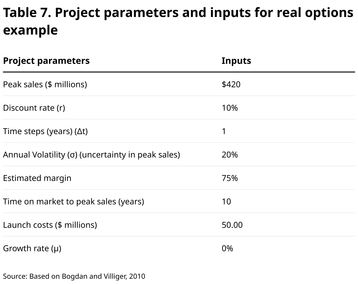
Let us briefly explore how each parameter can be determined:

• Peak sales: The estimation of peak sales involves conducting market research, analyzing comparable drugs in the market, and considering factors such as disease prevalence, potential market size, competition and pricing strategies. Market reports, industry experts, and historical sales data can provide valuable insights for estimating the potential revenue of the drug.

• Discount rate (r): The discount rate represents the cost of capital or the required rate of return. Typically, it is the firm’s cost of capital, as discussed in the rNPV section; if this value is not available, a rate can be determined from industry standards or investor expectations. Published financial models, investment bank analyst reports and industry benchmarks are often used to establish an appropriate discount rate. When a risk-neutral valuation approach is being employed, the risk-free rate should be used.

• Time steps (Δt): Time steps refer to the length of each period in the decision tree model. The choice of time steps depends on the specific characteristics of the drug’s development and market dynamics. Typically, shorter time steps are used for complex and rapidly changing markets, while longer time steps may be suitable for more stable markets.

• Annual volatility (σ): Annual volatility reflects the uncertainty or variability in the peak sales estimate. This parameter is determined by analyzing historical sales data of similar drugs, considering market dynamics, assessing the impact of potential factors such as regulatory changes or competition, and consulting industry experts. Statistical methods, such as calculating the standard deviation of past sales, can help estimate the annual volatility.

• Estimated margin: The estimated margin represents the profit margin or the percentage of revenue retained after deducting the costs of production, marketing and other expenses. It is typically determined based on industry benchmarks, cost structures, and profit projections. Financial analysis and expert insights are used to estimate the margin for the specific drug under evaluation.

• Time on market to peak sales: The time on the market to reach peak sales refers to the number of years from the drug’s launch to when it is expected to achieve its maximum sales potential. This parameter is based on market research, historical data of similar drugs, the expected adoption rate and factors influencing market penetration and acceptance.

• Launch costs: Launch costs encompass the expenses incurred during the initial launch of the drug, including marketing, sales, distribution and regulatory compliance. These costs are estimated by considering industry benchmarks, the scope of the launch strategy, market entry requirements and anticipated resource needs.

• Growth rate (µ): The growth rate represents the expected rate of sales growth after product launch toward peak sales. It can be influenced by factors such as market saturation, competition, new indications or markets and lifecycle management strategies. Market analysis, industry forecasts and expert opinions can inform the estimation of the growth rate.

It is important to note that these parameters are subject to uncertainty, and different scenarios and sensitivity analyses may be conducted to understand the impact of variations in the parameter values on the valuation outcomes. In particular, given the importance of volatility in option calculations, care should be taken to assess this value carefully and to explore the sensitivity of this input on the output values.

Step 2: Span the decision tree

Using these data and the formulae shown in Table 7 we can determine that for the CF project, u = 1.22, d = 0.82, p = 45 percent and (1–p) = 55 percent. We can now span the tree, following the approach used by Bogdan and Villiger (2010) as shown in Table 8.

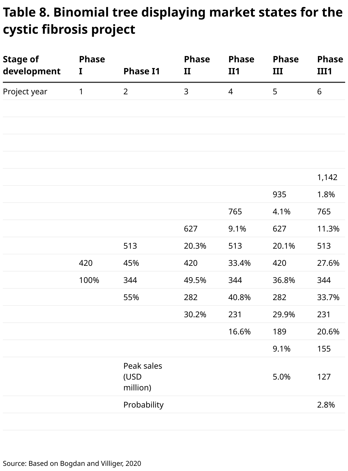
The Bogdan and Villiger approach spans a binomial tree for the peak sales estimate, which is determined by first developing an rNPV of the drug candidate and determining when peak sales are likely to occur. By incorporating the peak sales estimate as the starting point, the decision tree captures the potential upside and the subsequent strategic decisions that may influence the drug’s success and financial outcomes. Our drug candidate is indeed in its early clinical trial phase and the actual peak sales are uncertain. The decision tree allows for the exploration of different scenarios and decision points throughout the drug’s development lifecycle. It considers the potential risks, uncertainties and strategic choices that may impact the ultimate success and value of the drug.

The decision tree branches out at each decision point, considering factors such as trial results, regulatory approvals, market conditions and competitive landscape. By quantifying these factors probabilistically and incorporating the estimated peak sales, the decision tree provides insights into the value of the drug candidate under different possible outcomes. The goal of developing a decision tree in this way is to enable a more comprehensive analysis of the drug candidate’s value, incorporating both the uncertainty of its development path and the potential strategic decisions that can shape its future success. It provides a structured framework to assess the financial implications of different investment choices and helps stakeholders make informed decisions regarding resource allocation, licensing agreements or further development strategies

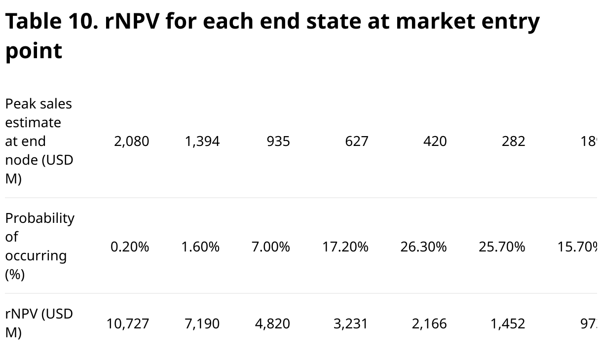
From Table 7, we estimate that there is a possibility of making up to USD 2,080 million in peak sales (at the highest value end node). However, this scenario is only likely to occur with a probability of 0.2 percent, which suggests that it is highly unlikely. Conversely, our most probable estimates are USD 420 million with a probability of 26.3 percent, and USD 282 million, with a probability of 25.7 percent. We also observe that for each node in a particular time step (each column) the probabilities add up to 100 percent. For this project, there are three decision points: the beginning of phase II, the beginning of phase III and the approval stage.

The probability of each end state is illustrated in Figure 11.

Figure 11. Probabilities of different end states for the cystic fibrosis project

Source: Based on Bogdan and Villiger, 2010

In analyzing the end states of our decision tree, we have uncovered a wide range of potential outcomes for the peak sales estimates of our drug candidate. This range spans from a high estimate of USD 2,080 million to a low estimate of USD 85 million. Within this spectrum, two key end states appear to be the most probable: USD 420 million and USD 282 million. These findings provide valuable insights into the financial performance of our drug candidate under different scenarios. The varying outcomes reflect the inherent uncertainties and risks involved in drug development, considering factors such as clinical trial results, regulatory approvals, market dynamics and competition.

The significance of these results lies in their implications for decision-making and strategic planning. By understanding the range of potential outcomes, we gain a clearer understanding of the risk-reward trade-offs associated with different development strategies, licensing agreements and resource allocations. This knowledge allows us to make more informed decisions about the optimal path to pursue.

Importantly, the analysis of end states demonstrates the value of utilizing a decision tree framework. It provides a structured approach for evaluating the potential financial outcomes of different strategic choices, enabling us to navigate the uncertainties inherent in early-stage biotechnology valuation. This comprehensive evaluation supports strategic planning, facilitates resource optimization and ultimately assists in maximizing the potential of your drug candidate.

Step 3: Calculate the rNPV of each end state

Once we have modeled the tree to the market entry stage, for the underlying (the peak sales of the drug), we use these peak sales estimates to develop the discounted cash flow of the project, to undertake the development of the compound and sum these up to determine the rNPV of the project/option for each node (Table 9).

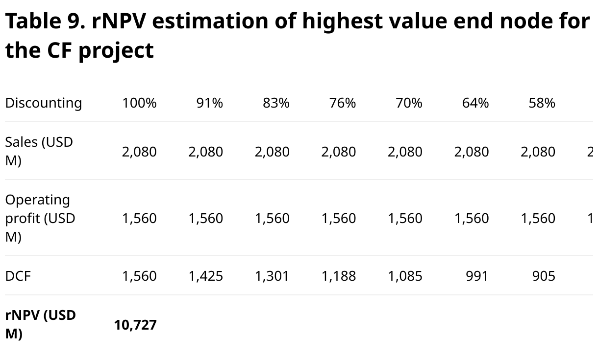
We then repeat this exercise for each end node to yield the rNPV values shown in Table 10.

Step 4: Extend the solution to the previous phases of the project

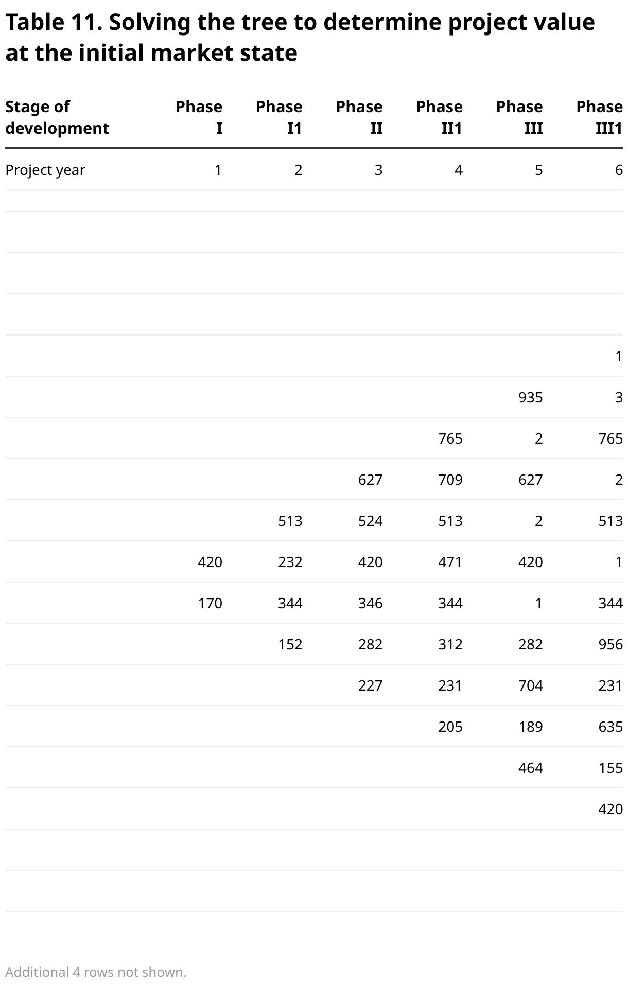
Now that we have the value of the end states of the option value, i.e., the value of undertaking the drug development project, we can work our way back through the tree to the previous time step (last year of phase III) to determine the rNPV during the development of the CF project and the value of the option at each node. In our calculations, we must account for the success rates of each phase and discount the values appropriately using the formula in Equation 5.

Equation 5. Calculation of project value

These calculations yield the values in Table 11.

When calculating the rNPV for each end state on a decision tree and extending the solution to previous phases of the project, several sanity checks can be conducted to ensure the accuracy and reliability of the results. These sanity checks serve as validation measures and help assess the reasonableness of the calculated values. Here are some common sanity checks:

• Sensitivity analysis: Varying key parameters, such as peak sales, discount rate, development costs or time frames, allows for an examination of how changes in these variables impact the rNPV. It helps identify which factors have the most significant influence on the valuation and can highlight areas of uncertainty or sensitivity.

• Comparison to historical data: Comparing the calculated rNPV with similar past projects or industry benchmarks can provide a reference point for evaluation. If the calculated values deviate significantly from historical data, it may indicate the need for further scrutiny or reassessment of underlying assumptions.

• Expert judgment: Seeking input from domain experts, such as experienced biotechnology professionals, industry consultants or advisers, can help validate the reasonableness of the rNPV estimates. Expert opinions can provide valuable insights into the specific dynamics and risks associated with the biotechnology sector.

• Consistency with market expectations: Assessing whether the calculated rNPV aligns with market expectations, investor perspectives or industry trends can serve as a reality check. If the valuation seems significantly out of line with prevailing market conditions or investor sentiment, it may warrant a reassessment of the inputs or underlying assumptions.

The contribution of conducting these sanity checks is to enhance the credibility and robustness of the valuation analysis. It helps identify potential errors, biases or inconsistencies in the model and allows for adjustments or refinements to be made. By incorporating various validation measures, decision-makers can have greater confidence in the rNPV results and use them as a basis for strategic decision-making, resource allocation or investment evaluations. Ultimately, this method helps in assessing the potential value and risk of early-stage biotechnology IP assets, facilitating informed choices and maximizing the value of the projects.

The approach that is detailed here is comprehensive and requires significant data gathering and computational effort. In other circumstances, for example in some technology licensing scenarios, a simpler assessment of the situation at each node may be adequate to develop a helpful model and to provide a financial value of the project. The binomial pricing method is flexible, adaptable to several option scenarios, and relatively transparent to the users of the end data; it provides a robust approach to valuing real options and can be used in a rigorous and complex fashion, as in this example, or in a more straightforward manner, depending on the situation.

Considerations when using real options

As mentioned earlier, the binary nature of drug development trials (success or failure) may mask other outcomes, which present project managers with a range of options to explore. For instance, clinical trial results may be overwhelmingly positive, triggering the expected next phase of trials. Conversely, they may fail from a safety or efficacy perspective in which case the project is abandoned. However, there are situations where the hypothesis under investigation is not proven by the data, but the researchers think that a redesign and refinement may be sufficient to run additional trials. Let us use a simple example to illustrate these points.

Figure 12: Decision tree for TumaBlok showing the range of viable options available

Source: Author based on Bogdan and Villiger, 2010.

In Figure 12, the red time steps (2, 4, 5, 6, 7, 8, 9 and 11) represent decision points for the project. The CEO would have to resolve each tree to estimate the project value at the start of the outset (year 1) for the complex TumaBlok decision tree. The CEO’s calculations must be based on defensible assumptions for peak sales estimates, growth rates and attrition levels during development for all products. These values must be sourced from well-established industry averages, sales values for similar drugs on the market and against comparable companies to BioTech in terms of profile (size and portfolio). The CEO must also be aware that the duration of trials may be longer than expected and consequently, may cost more. She must adapt her calculations accordingly. This example shows that the decision tree can be complex and may require careful resolution to ensure that all viable options are appropriately treated. For companies with several projects in their pipelines dedicated valuation tools and resources may be necessary to elucidate the value of individual projects and entire portfolios.

Industry experience in using real options – benefits and challenges

Many valuation experts believe that real options provides the closest approach to the economic truth of the set of techniques that are reviewed in this guide. The explicit consideration of growth and termination options is useful and can help frame insightful discussions internally and provide a framework for articulating the value of an asset or a technology in a negotiation setting. However, real options analysis relies on complicated techniques and is unfamiliar to many people, including many senior managers in the biotechnology and pharmaceutical industries. The inclusion of growth options can lead to values that exceed those generated by NPV approaches and to rigorous questioning, hence the suggestion in this guide to apply the binomial approach. In the pharmaceutical industry, the fact that rNPV is a well-understood approach has led to its dominance, although many firms have at least in some situations used real options valuation approaches over the past 10 to 15 years. The real options method has some challenges but also great potential, and its use is likely to increase over the next decade.